In this post I’m going to diverge from the usual topic of finance and focus on a powerful feature of the Google Sheets, named functions. I’m going to demonstrate how to create a named function to boost your productivity and use it in conjunction with LAMBDA functions. When I was working as a teacher, I was faced with a problem to calculate the final grade of hundreds of students based on multiple assignments, each with a different percentage weighting. Upon searching, I could only find some convoluted ways to achieve it. In the spirit of automating everything and solving problem my own way, I made a custom function so all the calculations can be done with a single formula. And I’m going to show you step-by-step how to create this function on your own Google Sheet, using the onion method. (You can access the template with the link at the bottom of this post!)
If you’re new to the idea of named functions, simply think of it as specialized formulas designed to solve a specific need when your vanilla formulas just don’t cut it. Named functions can be very handy when you need to automate a workflow that involves many steps. With the easy-to-use interface, you can combine all the steps into a single function, provide description of each argument in the formula so users of your formula can learn to use it in no time, not to mention that you can import named functions to a new sheet so it’s really a great tool for organizations. Refer to Google’s documentation for more info.
Anyway, let’s get to the meat of topic. To calculate the weighted total of multiple students based on their marks on multiple assignments, we need the following information:
- The weight each assignment carries (in percentage)
- The full mark of each assignment
- The mark each student got in each assignment

Then, go to Data in the menu, select “Named Functions”. Click on “Add new function”. You’ll be asked to enter the function name, argument placeholders, formula definition and additional details.
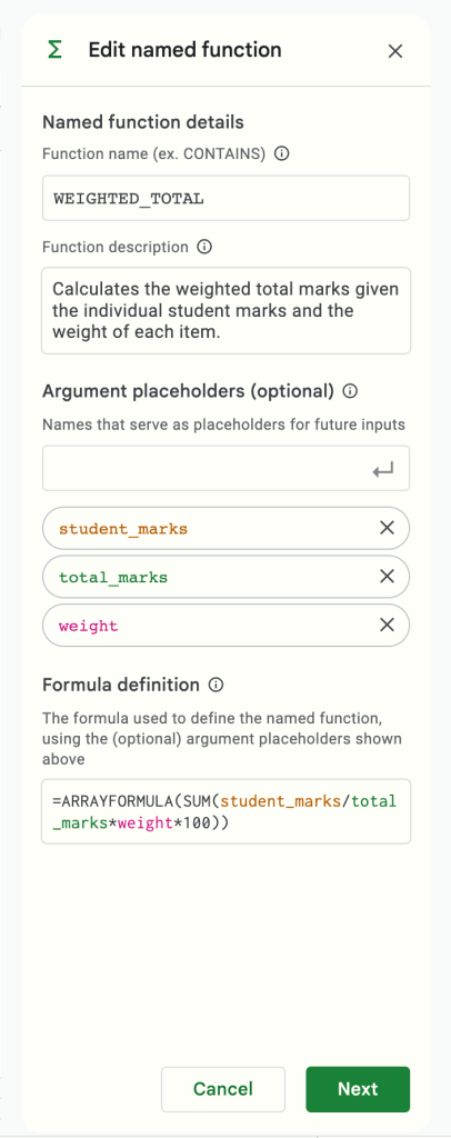
In this case, the function name is WEIGHTED_TOTAL
Please note that the function names must meet the following requirements:
- Can’t be named the same as a built-in Sheets function like
SUM. - Can’t be named
TRUEorFALSE. - Can’t be in either “
A1” or “R1C1” syntax. (e.g. if you give your function a name like “A1” or “AA11,” you get an error.) - Can’t start with a number.
- Must be shorter than 255 characters.
- Must have no spaces.
- Must have no special characters except for underscores.
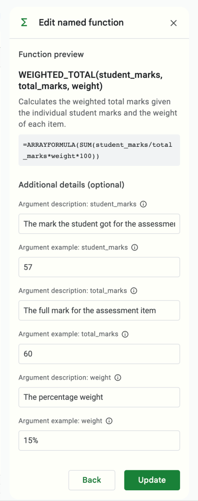
After you’ve entered all the required information, click “Update”. Then the function is live!
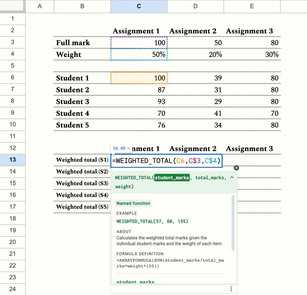
Now in the space below the data, insert a table of 5 rows to calculate the weighted mark of each students’ assignment. First, I’ll apply the formula to Student 1 like the screenshot below. Note that the row reference of the full mark and the weight are locked so that copying down the formula will not mess up the calculation. Also, I’ve highlighted the cell C13 in color to indicate that it has a formula to prevent accidental overwrites.
Then, copy down the formula to cell C17 and drag the range C13:C17 to column E. The cells should populate with the correct weighted mark.
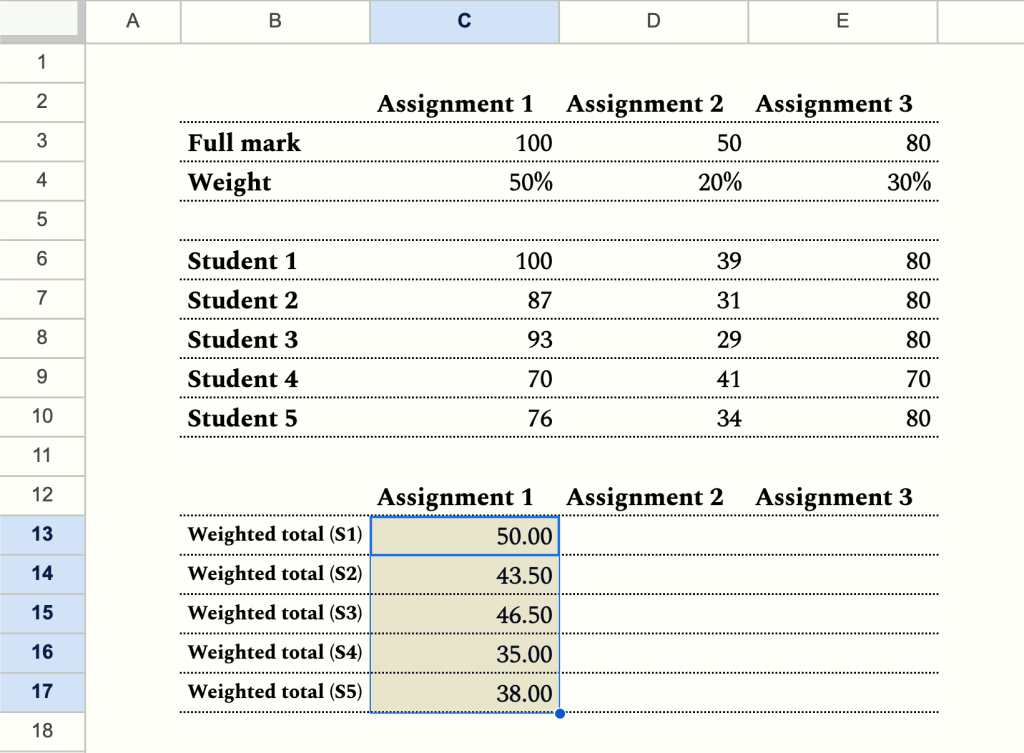

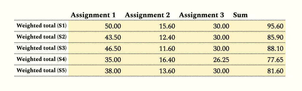
The next step would be to sum up the weighted marks so each student would get a weighted total (out of 100).
We already finished the calculation part. However, with hundreds of students, the number of data points can be overwhelming. So we need to automate as much as possible. Therefore, we’ll use ARRAYFORMULA on the named function we’ve just created.
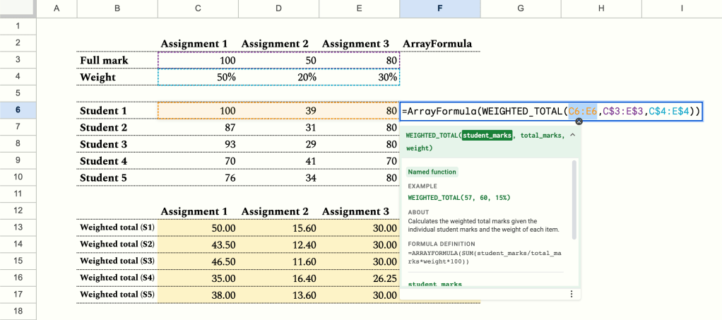
We’ll copy the formula in cell C13 to cell F6, then using the shortcut Cmd+Shift+Enter for Mac or Ctrl+Shift+Enter for PC, turn the formula into an ARRAYFORMULA. Then, we’ll extend the student_marks argument into a range (C6:E6). And voila! We’ve successfully calculated the weighted total of a student using a single formula! Now, does that mean the next step is to copy the formula down? Well, remember we need to automate as much as possible? Having hundreds on ARRAYFORMULA probably isn’t a good idea. Would the solution be applying ARRAYFORMULA on the already existing ARRAYFORMULA i.e. nested ARRAYFORMULAs then? Not impossible, but I prefer to use a more elegant solution, i.e. the BYROW function.
The BYROW function in Google Sheets operates on an array or range and returns a new column array, created by grouping each row to a single value. You can read more about it and Google’s documentation.

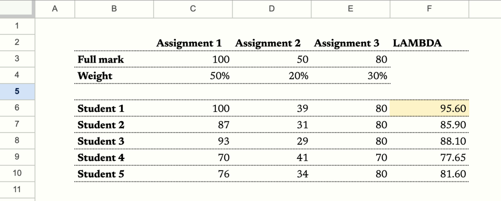
With the BYROW function, we have now successfully automated the calculation of weighted totals of the entire row of students. When applying this solution to my actual grade sheet, I would define the LAMBDA as an open-ended range (e.g. C6:E) so that whenever I add a new student at the bottom of the sheet, the formula will automatically calculate a weighted total for that student.
If you want to play with the function and modify it yourself, click here to generate a copy of the sheet. I hope you enjoy this tutorial and have a great day!
J
I hope you enjoy this tutorial as much as I enjoy writing it. If you’re into organizing your life, be sure to check out the ZestFi Stock Portfolio Tracker. Not your typical Google Sheet template, the ZestFi Stock Portfolio Tracker lets you easily track all your stocks even if you have multiple accounts, own different types of assets, and hold multiple currencies! This tracker makes use of the GOOGLEFINANCE API to fetch stock price updates and provides powerful analytics presented in a ultra clean dashboard, helping you make the best investment decisions. Say goodbye to the hassle of going back and forth between different apps and website to manage your investments, and say hello to ZestFi!
