ZestFi

Welcome to the world of Sharpe ratios—a powerful tool in portfolio management that helps investors assess the return of an investment relative to its risk. In this tutorial, we’ll leverage the magic of Google Sheets to calculate Sharpe ratios and compare the performance of Apple stock (AAPL) against the S&P500 over the last three years. We’ve crafted a Google Sheets template to simplify the process, and we’ll guide you through each step.

Accessing the Template

To get started, access our Google Sheets template by clicking the button below. Follow the instructions provided to understand how to use this dynamic tool for Sharpe ratio calculations.

• Download the Google Sheets Template: We’ve created a spreadsheet that will be continually updated with examples and functionalities. To access it, simply click the button above.
• Access to the Sheet Forever: Once you’ve downloaded it via our Gumroad page, you’ll have unlimited access to the template. You can also make a copy of the sheet to experiment with various performance metrics using your own portfolio data.
• Stay Updated: The best part? We’ll keep updating the spreadsheet with new examples and features, so you don’t have to worry about a thing.
• Add a Shortcut to Your Google Drive: To make your life even easier, you can add a shortcut to this invaluable tool in your Google Drive. Here are the instructions from Google on how to do it.

Without further ado, let’s dive into the tutorial!

Pulling S&P500 Data

To begin, we’ll pull the data of the closing price of S&P500 going back three years from GOOGLEFINANCE. Since we want to make the sheet more dynamic, we’ll assign cell I13 as the input cell for the number of years so whenever you want to adjust it, you can simply change the number in that cell and the data automatically refreshes. So in cell A2, insert this formula:

==GOOGLEFINANCE(".INX","price",TODAY()-$I$13*365,TODAY())

Explanation:

• .INX: Ticker symbol for the S&P500.
• price: Fetching the closing prices.
• TODAY() - $I$13 * 365: Specifying the date range based on the user-defined number of years in cell I13.

Calculating Daily Price Changes

Then we want to calculate the day-to-day price changes in percentage terms. Typically, you can do it by using (new price-old price)/old price formula, then copy down the formula to the bottom of the page. However, since the length of the data might change depending on the input cell – cell I3, so we have to come up with a formula that can dynamically handle the changing length of the dataset. Therefore, we’ll use LAMBDA in cell C4.

=ARRAYFORMULA(IF(B4:B<>"",LAMBDA(new,old,(new-old)/old)(B4:B,B3:B),))

Explanation:

• The LAMBDA function handles dynamic data length.
• new: Represents the new day’s closing price.
• old: Represents the previous day’s closing price.

Pulling AAPL Data

Now that we have set up the market data of S&P500 on the first 3 columns, we can apply the same thing on the Apple stock on the next 3 columns. In cell D2, enter this:

=GOOGLEFINANCE(D1,"price",TODAY()-$I$13*365,TODAY())

In cell F4, enter this:

=ARRAYFORMULA(IF(E4:E<>"",LAMBDA(new,old,(new-old)/old)(E4:E,E3:E),))

Reference Cells

Then, let’s add some reference cells that return the last closing price of S&P500 and AAPL In cell I16, enter this:

=XLOOKUP(MAX($A$3:$A),$A$3:$A,$B$3:$B,)

And in cell I17, enter this:

=XLOOKUP(MAX($A$3:$A),$A$3:$A,$E$3:$E,)

And we’ll need to get the row number of the last row as well for reasons you’ll see later in the post. In cell J16, enter this:

=ROW(XLOOKUP(MAX($A$3:$A),$A$3:$A,$B$3:$B,))

And in cell J17, enter this:

=ROW(XLOOKUP(MAX($A$3:$A),$A$3:$A,$E$3:$E,))

Sharpe Ratio Calculations

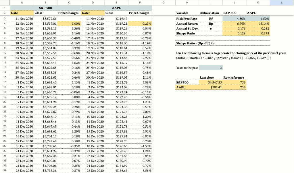
In order to calculate the Sharpe ratio, we’ll need the Risk Free Rate. In this example, let’s use 4.50%. Standard deviation of the excess return.

In cell J4, we’ll use this formula to calculate the annual return of S&P500:

=((INDIRECT(ADDRESS(J16,2))/B3)^(1/$I$13))-1

Likewise, in cell K4, enter this to calculate the return of AAPL:

=((INDIRECT(ADDRESS(J17,5))/E3)^(1/$I$13))-1

For the annual standard deviation, we’ll use this formula in cell J5 and K5 respectively:

=STDEV.P(C4:C)*252^0.5

=STDEV.P(F4:F)*252^0.5

Then, we can calculate the Sharpe ratio respectively.

=(J4-J3)/J5

=(K4-K3)/K5

Conclusion

Congratulations! You’ve successfully navigated the complexities of Sharpe ratios using Google Sheets. The calculated Sharpe ratios serve as valuable metrics for evaluating the risk-adjusted performance of AAPL and the S&P500. Remember, the higher the Sharpe ratio, the better the risk-adjusted return. Happy investing!